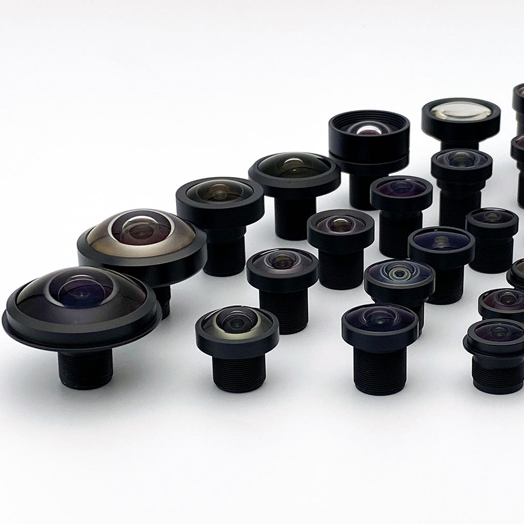

Machine Vision Lens Metrology Guide

How to Read MTF Curves: Contrast, Spatial Frequency, and Sensor Matching for Machine Vision

MTF is contrast transfer versus spatial frequency. This guide covers both chart formats, sagittal and tangential curves, field-position data, sensor matching by pixel pitch, and the difference between design MTF and measured MTF.

By Commonlands engineering team · Updated July 2026 · 18 min read

An MTF test bench with a collimator, goniometer stage, and a lens under test

An MTF curve plots how much contrast a lens transfers from scene to sensor, on a scale of 0 to 1, against spatial frequency in line pairs per millimeter (lp/mm). To read one: calculate the Nyquist frequency of your sensor, read the lens contrast at 0.5× to 0.7× of that frequency at the field positions your algorithm uses, and check that the sagittal and tangential curves stay close together. A lens that looks strong at the center can still fall short at the edge of the image circle, so field-position data matters as much as the on-axis curve.

MTF does not report distortion, chromatic aberration, or focus stability, so treat it as the first screen in lens selection rather than the verdict. This guide explains both chart formats, every axis and curve label, how MTF connects to sensor resolution, and how measured MTF from a Trioptics ImageMaster HR2 differs from the design curve in a datasheet.

What is MTF?

MTF, the modulation transfer function, is the ratio of image contrast to object contrast as a function of spatial frequency, measured in line pairs per millimeter (lp/mm). An MTF of 1.0 means the lens transfers full contrast at that frequency; 0.3 means 30% survives. Every MTF value is tied to a specific frequency, field position, and test condition.

MTF is formally defined for a target with sinusoidal intensity modulation. Contrast at each spatial frequency is defined by the Michelson formula, and the lens images the pattern with some blur, so the contrast in the image is lower than in the object; the ratio of the two, taken at each spatial frequency, is the MTF. Bench instruments rarely image an actual sine pattern. They derive MTF from a slanted edge or slit response through a Fourier transform, which is mathematically equivalent to the sine-wave definition. A square-wave bar target measures a related but distinct quantity, the contrast transfer function (CTF), which reads higher than MTF at the same frequency because it carries the fundamental plus odd harmonics (Coltman); Smith's Modern Optical Engineering (4th ed.) explicitly distinguishes sine-wave MTF from square-wave bar-target response, so a bar-target contrast ratio should be labeled CTF, not MTF.

C = (L_max − L_min) / (L_max + L_min) MTF(f) = C_image(f) / C_object(f) L_max and L_min are the brightest and darkest values of the sinusoidal test pattern. f is spatial frequency in lp/mm. At f = 0 the normalized MTF is 1.0 by definition.

One line pair is one dark bar plus one adjacent bright bar. A spatial frequency of 50 lp/mm packs 50 such pairs into one millimeter on the sensor, so higher lp/mm means finer detail. A 10µm feature on the sensor corresponds to roughly 50 lp/mm; a 5µm feature to roughly 100 lp/mm. A lens can have an MTF of 0.7 at 100 lp/mm and 0.2 at 300 lp/mm. Both numbers describe the same lens, and which one matters depends on your pixel pitch and the feature size you need to detect.

In-focus, well-corrected MTF curves generally slope downward with increasing frequency because every lens blurs light over a finite spot. Fine patterns wash out first, since their period approaches the scale of that blur. Once contrast reaches zero at the cutoff frequency, no detail passes at all, regardless of sensor resolution. That monotonic falloff is not universal: defocused or strongly aberrated systems can produce non-monotonic curves that dip to zero and rebound at higher frequencies, an effect known as spurious resolution. Stopping down the aperture usually raises MTF by shrinking aberrations, then lowers it again as diffraction grows; the f-number guide covers that tradeoff, and many machine vision lenses measure best one to two stops down from wide open.

Why MTF decides detection reliability

Contrast the optics lose never reaches the pixel. Software sharpening amplifies whatever signal and noise remain; it cannot recover a bar pattern the lens delivered at zero contrast. When MTF at your working frequency drops below roughly 0.2 to 0.3, sensor noise competes with the remaining signal and detection becomes unreliable.

MTF is also field-dependent. The same lens typically measures higher at the center of the image than at the edge, so a complete characterization reports curves at several image heights, not one headline number. That field behavior gets its own chart format, covered below.

A workstation monitor showing measured MTF curves of contrast versus spatial frequency
Sagittal and tangential curves fall as spatial frequency rises.

How do you read an MTF curve?

Identify the plot format first. MTF vs spatial frequency fixes the field position and sweeps detail fineness; MTF vs image height fixes the spatial frequency and sweeps from center to corner. Then read the contrast value at the frequency your sensor samples, at the field positions your algorithm uses, on both sagittal and tangential curves.

The frequency format answers one question: at a given field position, how does contrast change as detail gets finer? The field format answers the complementary one: at a given detail level, how does contrast change from center to edge? Sensor matching leans on the first format. Field-uniformity checks lean on the second. A datasheet that provides only one of them is half a specification.

Reading the frequency axis

On an MTF vs spatial frequency chart, the x-axis runs in lp/mm and the y-axis runs from 0 to 1.0, or 0 to 100% on some datasheets. At zero frequency the normalized curve starts at 1.0, then falls as frequency increases. The information is in how fast it falls and where it sits at the frequencies you care about. Datasheets typically overlay curves for several field positions: on-axis, around 0.7 field, and full field, each with sagittal and tangential traces. Higher and flatter is better at the frequency band your application samples.

Chart feature What it means Why engineers care
Spatial frequency (lp/mm) Line pairs per millimeter on the sensor; a measure of detail fineness Must be read against the sensor's Nyquist limit to confirm the lens is not the resolution bottleneck
MTF value (contrast) Ratio of image contrast to object contrast, from 0 to 1 Sets how reliably an algorithm detects features at that detail level; low contrast raises miss rates
Image height (mm) Distance from the optical axis to the measurement point Center and edge performance are separate facts; the corner of your sensor sets the image height to verify
Sagittal curve (S) MTF for features oriented radially, toward or away from the axis Separation from the tangential curve reveals astigmatism at that field height
Tangential curve (T) MTF for features perpendicular to the radius Large S-T separation means sharpness depends on feature orientation, which breaks orientation-agnostic detection
MTF50

MTF50 is the spatial frequency where the curve crosses 0.5. It is a useful single-number summary for comparing lenses quickly, and it correlates with perceived sharpness in photographic use. It is not a substitute for reading the curve at your own frequency: a lens with a high MTF50 and a steep rolloff can still sit below 0.3 at the frequency an inspection task needs.

Cutoff frequency

The cutoff is the frequency where MTF reaches zero and no spatial information passes. Diffraction sets the theoretical ceiling for a given aperture and wavelength; residual aberrations pull the curve lower but never extend the cutoff beyond it.

f_cutoff = 1 / (λ × f/#) 546nm at F/4: 1 / (0.000546mm × 4) ≈ 458 lp/mm λ is wavelength in mm. The formula applies to incoherent illumination. An aberrated lens loses useful contrast well before this ceiling.

If a lens holds usable contrast to 400 lp/mm and your sensor needs 250 lp/mm, there is headroom. If contrast collapses by 150 lp/mm and the sensor samples to 200 lp/mm, the lens is the limiting component. The diffraction limit section of the spatial resolution guide works through the aperture and wavelength math in detail.

What do sagittal and tangential MTF curves mean?

Sagittal curves plot contrast for features oriented radially, along the line from the image center outward. Tangential curves plot contrast for features perpendicular to that radius. The two are identical on-axis for a perfectly centered, rotationally symmetric design. On a measured unit, an on-axis S-T split points to asymmetry in the assembly, such as element decenter or tilt, though test-fixture misalignment can produce the same signature, so verify the setup before attributing it to the lens. At off-axis positions, separation between the sagittal and tangential curves indicates astigmatism at that image height.

A wheel makes the orientation concrete: sagittal features run like spokes, tangential features run like the rim. An off-axis point in an astigmatic lens focuses spoke-oriented detail and rim-oriented detail at slightly different distances, so one orientation is sharp while the other is soft at any single focus setting. That is why each field position on an MTF chart carries two traces instead of one.

The separation is a diagnostic signal. Curves that track each other across the field indicate a lens that resolves detail equally in all orientations. A widening gap toward the edge means off-axis aberrations, primarily astigmatism, are building toward the image boundary; the lens aberrations guide explains the underlying mechanisms. The practical consequences are specific: round holes and particles image as ellipses near the corners, and edge-detection thresholds tuned at one orientation misfire at another. When feature orientation in your application is fixed, verify the lower of the two curves at your operating frequency, because that is the orientation-worst-case contrast the algorithm will see.

How do you read MTF vs field-position curves?

An MTF vs field curve plots contrast at a fixed spatial frequency against image height, the distance from the optical axis in millimeters. The center of the image sits at 0mm; the maximum is the half-diagonal of the target sensor format. A flat curve means uniform performance; a steep drop marks the radius where correction runs out.

Convert your sensor geometry to image height before reading the chart. A 1/1.7" format sensor has a diagonal of approximately 9.4mm, so its corner sits at an image height of about 4.7mm. Format names do not map exactly to millimeter dimensions, so take the diagonal from the sensor datasheet rather than the format label; the sensor size and lens compatibility guide covers image circle coverage and format math.

Two curve shapes deserve different responses. A moderate, smooth decline that still clears your contrast threshold at the corner image height is normal behavior for a well-corrected design. A cliff at a specific radius is an optical design boundary: performance degrades rapidly beyond it, and pairing that lens with a sensor whose corners reach past the cliff produces soft corners no focus adjustment will fix.

Field uniformity matters because defects do not appear on the optical axis by appointment. In most inspection systems, features land anywhere in the frame, and the corner is a routinely used region rather than an edge case. Wide-angle designs face the hardest field demands, since the off-axis optical path steepens quickly with field angle. A 4mm lens covering 98° needs field MTF verified at multiple image heights, not a center measurement extrapolated outward.

CIL560 4mm C-mount lens mounted on a 1/1.7-inch machine vision camera for full-field evaluation
A 4mm C-mount lens on a 1/1.7" camera. With a 9.4mm sensor diagonal, corner performance means MTF verified out to an image height of about 4.7mm.

How do you match lens MTF to sensor pixel pitch?

Calculate the sensor's Nyquist frequency, 1000 divided by twice the pixel pitch in µm, then read the lens MTF at 0.5× to 0.7× of that frequency at every field position your algorithm uses. A lens holding MTF at or above 0.3 across that band is rarely the resolution bottleneck for that sensor.

Nyquist (lp/mm) = 1000 / (2 × pixel pitch in µm) 1.85µm pixel → 270 lp/mm 3.45µm pixel → 145 lp/mm 5.86µm pixel → 85 lp/mm Nyquist is the frequency at which adjacent pixels sample opposite phases of a line pair: the sensor's sampling ceiling, not a performance target.

The 0.5× to 0.7× band exists because real sensors give up resolution before Nyquist. Bayer color sensors lose fine detail to demosaicing, anti-aliasing filters deliberately suppress contrast near Nyquist to prevent artifacts, and noise dominates as contrast approaches zero. For a 1.85µm sensor, that band spans roughly 135 to 190 lp/mm. A lens above 0.3 there feeds the sensor usable contrast at the detail levels it can actually digitize; a lens already below 0.2 at half-Nyquist wastes the sensor's pixel count.

Setting the contrast threshold

No universal MTF threshold guarantees reliable machine vision. The threshold follows from the algorithm's contrast sensitivity, the lighting, and the acceptable miss rate. The values below are working starting points, not guarantees.

Application Typical frequency of interest Starting MTF target Notes
1D barcode reading 10–40 lp/mm 0.4 at the narrow-bar frequency Wide bars are forgiving; high-density Code 128 narrow bars are not
2D barcode / QR 20–60 lp/mm 0.3 across the symbol area A code at the frame corner must still decode, so field uniformity matters
OCR 40–80 lp/mm 0.3 at the stroke frequency Printed character strokes typically span roughly 100–400µm on the object, depending on point size and print process
Surface defect inspection Set by minimum defect size 0.3 at the defect frequency Defect size × magnification gives feature size on sensor, which gives frequency
Dimensional measurement 50–150 lp/mm 0.4 at half Nyquist, uniform across the field Sub-pixel edge detection also requires the distortion budget checked separately
AI / CNN object detection 20–60 lp/mm 0.3 at mid frequencies, field uniform CNNs tolerate soft optics better than edge-based code, but train/deploy optics should match
Robotic guidance Application-dependent 0.3 at the required feature frequency Corner MTF is relevant when targets cross the full field

Relating image-space frequency to feature size in the scene

MTF is specified in the image plane, so object-space features must be converted through magnification before the chart means anything. Image-space frequency equals object-space frequency divided by the magnification m. At m = 0.1, a 10 lp/mm pattern in the scene lands on the sensor at 100 lp/mm, so that is the frequency to read on the curve. Magnification follows from focal length, sensor size, and working distance; the focal length guide and the field of view calculator give the numbers for your geometry.

Aperture belongs in the same calculation. Many C-mount lenses carry an adjustable iris, and stopping down one to two stops often raises off-axis MTF because residual aberrations shrink faster than diffraction grows. M12 lenses typically use a fixed aperture, so the aperture point on the MTF curve is chosen at purchase rather than tuned at the fixture.

What is the difference between design MTF and measured MTF?

Design MTF is computed from the lens prescription in optical design software and assumes every element sits at its nominal position. Measured MTF is instrument data from a physical lens and includes decenter, tilt, spacing error, and glass variation from manufacturing. As-built MTF is typically lower than the design curve, so acceptance decisions should use measured data.

The gap between the two comes from the tolerance stack. Element decenter and tilt, airspace errors, refractive index variation between glass melts, and surface irregularity each take a bite out of the nominal curve, and tolerance analysis predicts a distribution of as-built performance rather than a single line (Smith, Modern Optical Engineering, 4th ed.). Two units of the same design can therefore measure differently, which is the argument for testing individual lenses rather than trusting a representative curve.

Slanted-edge testing

Slanted-edge measurement, standardized in ISO 12233, images a high-contrast edge at a slight angle, derives the edge spread function, differentiates it into the line spread function, and Fourier-transforms that into MTF. It runs at any working distance with a printed target and controlled lighting, which makes it well suited to production checks and application-distance validation. Its limit is coverage: it reports MTF where the edge sits, so full-field data requires deliberately placing targets across the frame.

Bench measurement on the Trioptics ImageMaster HR2

Optical benches measure the lens itself at controlled field angles and wavelengths. The Trioptics ImageMaster HR2 is the Commonlands measurement reference. A standard report covers MTF versus spatial frequency and MTF versus field, measured with a photopic weighting at infinity conjugate over 9 field points across 3 azimuths, plus EFL on axis and versus field, distortion at 21 points along one axis, lateral and longitudinal chromatic aberration at 480nm, 546nm, and 644nm, astigmatism as an MTFS versus MTFT surface map, and field curvature across the field, with on-axis through-focus MTF available on request.

On this bench the MTF is traceable to international standards through PTB, the German national metrology institute, and the EFL is traceable to NIST. That traceability is what lets a report back incoming inspection and lot acceptance rather than a subjective pass or fail. Commonlands uses the instrument to measure its M12 lens designs, and the $199 test report is open to customer-supplied lenses; near-infrared users can request MTF at 850nm and 940nm.

Commonlands M12 lenses staged on the Trioptics ImageMaster HR2 optical bench for MTF and EFL measurement
Lenses staged on the Trioptics ImageMaster HR2. The bench measures each lens directly at set field angles and wavelengths, so the report reflects the as-built unit.
Measured MTF performance chart from a Trioptics ImageMaster HR2 machine vision lens test report
A measured MTF chart from an ImageMaster HR2 report. As-built curves include the manufacturing tolerances that a design-software plot leaves out.

Test conditions that must be reported

MTF data is only valid for the conditions under which it was taken. Before comparing two charts, confirm the working distance, the aperture, the wavelength or illumination band, the field positions tested, the focus condition, and the temperature when the deployment is thermally demanding. Each variable shifts the curve.

Comparing curves from different conditions

A curve at F/2.0, infinity focus, 546nm cannot be compared directly against a curve at F/5.6, 500mm conjugate, broadband white light. Both are valid measurements of different operating points. A vendor showing only center MTF, wide open, at one wavelength is presenting the most favorable number, not the number your fixture will see.

MTF measurement options compared

Three routes produce MTF data, and they do not measure the same thing. In-house slanted-edge testing to ISO 12233 reports system-level MTF for the price of a target and software; the Commonlands Trioptics ImageMaster HR2 service returns component-level lens curves at $199 per lens; buying bench time or equipment from a metrology house suits high-volume inspection or an internal lab. Pick the cheapest route that isolates the variable you actually need to qualify.

Approach What it measures Relative cost Best fit
In-house slanted-edge (ISO 12233 chart plus analysis software) System-level MTF: lens, sensor, and ISP together, at your working distance Lowest; a printed target and software on hardware you already own Pass/fail checks on your own production line
Commonlands MTF testing on the Trioptics ImageMaster HR2 Component-level lens MTF on a calibrated bench, vs frequency and vs field at 9 positions across 3 azimuths $199 per lens, no capital outlay Traceable incoming inspection or lot acceptance without owning a bench
Dedicated lab equipment or bench time from Trioptics or Optikos Component-level MTF plus wider optical metrology, scaled to your throughput Highest; capital equipment or per-hour bench service High-volume incoming inspection or an internal metrology lab

If the sensor and ISP are part of what you are qualifying, in-house slanted-edge data answers the question. If you need to compare bare lenses against a datasheet curve, only component-level bench MTF settles it, because a system measurement folds in a sensor you cannot separate out afterward.

What can MTF not tell you on its own?

MTF quantifies contrast transfer and nothing else. It does not measure distortion, chromatic aberration, relative illumination, working-distance dependence, focus stability, or mechanical fit. A lens can pass an MTF screen and still fail dimensional measurement because of distortion, or fringe color under broadband light. Treat MTF as one axis of a complete characterization.

Distortion

Distortion maps straight lines in the scene to curved lines in the image while leaving contrast untouched, so a high-MTF lens can still carry several percent of barrel or pincushion error. Dimensional measurement and any task that depends on accurate spatial relationships need the distortion specification checked on its own; the lens distortion guide covers types, calibration, and selection thresholds.

Chromatic aberration

Lateral chromatic aberration shifts color channels relative to each other across the field, producing fringing at edges. Broadband or single-wavelength MTF averages over the effect or misses it, so a lens can post acceptable white-light MTF and still confuse color-sensitive algorithms. For multi-wavelength illumination, request per-wavelength MTF or review the chromatic specification separately, as explained in the chromatic aberration section of the aberrations guide.

Working-distance dependence

MTF reports are taken at a specific conjugate, often infinity. At a short working distance the aberration balance shifts and the curve changes, sometimes substantially. For close-range inspection, confirm the test distance matches the application or request close-conjugate data; the working distance guide explains how distance interacts with the rest of the optical budget.

Focus stability

Peak MTF assumes focus at the optimum, and small focus errors cost contrast quickly at high spatial frequencies. Thermal expansion, vibration, and mechanical settling all move focus after setup. A lens with an excellent bench curve still underperforms in a system that has not validated focus retention; the camera focusing guide covers establishing and verifying stable focus.

The explicit rule: a lens that fails MTF at your frequency and field position is out, but a lens that passes has cleared one gate of several. Distortion, chromatic behavior, working-distance range, focus stability, sensor coverage, and mount compatibility each require their own verification before the design freezes.

What are common mistakes when reading MTF charts?

Five mistakes recur in lens selection: comparing curves taken under different test conditions, accepting center-only data for a full-frame task, ignoring corner performance, treating a megapixel rating as measured contrast, and reading MTF in isolation from distortion and field curvature. Each one produces a lens that passes on paper and underperforms in the fixture.

  1. Comparing charts from different test conditionsWorking distance, aperture, wavelength, and field coverage all change the curve. Normalize the conditions before ranking two lenses against each other, or you are comparing operating points rather than optics.
  2. Trusting on-axis data for a full-frame taskCenter MTF is usually the lens's best case. Without curves at 0.7 field and full field, most of the image area is unspecified. Ask for the field data before committing.
  3. Ignoring corner performanceThe corner is the worst-measuring point and a routinely used one. When corner data is absent, assume it sits below whatever is shown, especially on wide-angle designs.
  4. Confusing megapixel rating with measured MTFA 12MP label describes intended sensor coverage. Two 12MP-rated lenses can deliver very different contrast at the frequencies a 12MP sensor samples. Only the measured curve settles it.
  5. Reading MTF in isolationMTF says whether an edge is sharp when it arrives. Distortion says whether it arrives in the right place, and field curvature says whether center and edge can focus simultaneously. Dimensional measurement needs all three inside tolerance.

MTF-tested lenses and the MTF testing service

Commonlands measures M12 lens designs on the Trioptics ImageMaster HR2, so selection decisions can rest on measured curves rather than design plots. Three MTF-tested options cover the demand space: the CIL560 4mm C-mount for wide-field coverage, the CIL561 6mm C-mount for a tighter field on the same 1/1.7" format, and the CIL122 IR-corrected 12mm M12 for near-IR work. The test service applies the same instrument to lenses you supply.

Procurement note

Commonlands stocks a broad range of M12 lens variants in the US, with C-mount and filter inventory alongside. Orders placed before 12 PM PST ship same day from San Diego, CA. ISO 9001:2015 certified.

How to read an MTF chart in 60 seconds

This sequence works for both chart formats and turns any lens datasheet into a pass, fail, or ask-for-more-data decision.

  1. Compute NyquistNyquist (lp/mm) = 1000 / (2 × pixel pitch in µm). Write it down, along with the 0.5× to 0.7× band.
  2. Convert your sensor corner to image heightHalf the sensor diagonal in mm is the farthest field position your frame uses.
  3. Find the curve for that field heightIf only center MTF is shown, treat the datasheet as incomplete and request field data.
  4. Read contrast in your frequency bandAbove 0.3, or your application threshold, the lens is a candidate at that field position.
  5. Compare sagittal and tangential tracesA small edge separation indicates mild astigmatism; a large gap demands a check against your feature orientation.
  6. Confirm coverage to the cornerThe curve must extend to your corner image height, not stop at the half-way field position.
  7. Check the test conditionsWorking distance, aperture, and wavelength must be representative of the application, or the curve needs re-measurement at your conjugate.
  8. Verify distortion and chromatic data separatelyMTF captures neither, and both can disqualify a lens that passed every step above.

A lens that clears all eight steps is a candidate, not a selection. Focus stability and mechanical fit still need verification in the fixture before the design freezes.

A machine vision lens clamped in a goniometric holder on an MTF tester bench
The bench rotates the lens to measure MTF across the field.

Frequently asked questions

What is MTF in a lens?

MTF, the modulation transfer function, is the ratio of image contrast to object contrast at a given spatial frequency, expressed in line pairs per millimeter (lp/mm). An MTF of 1.0 means full contrast transfer; 0.3 means 30% survives. It is a curve across frequency and field position, not a single sharpness score.

How do you read an MTF chart?

Identify the format first: MTF vs spatial frequency plots contrast against lp/mm at fixed field positions, while MTF vs image height plots contrast against field position at fixed frequencies. Read the contrast at the frequency band your sensor samples, at the field positions your algorithm uses, and compare sagittal and tangential curves for astigmatism.

What is the difference between MTF vs field and MTF vs spatial frequency?

MTF vs spatial frequency shows how contrast falls as detail becomes finer, which matches a lens to pixel pitch. MTF vs field shows how contrast at one frequency changes from center to corner, which reveals field uniformity. A complete evaluation uses both, because strong on-axis MTF does not imply uniform corners.

What does sagittal vs tangential mean on an MTF plot?

Sagittal curves describe contrast for features oriented radially, like spokes pointing at the image center. Tangential curves describe features perpendicular to the radius. They are identical on-axis for a centered design; on a measured unit, an on-axis split points to asymmetry in the assembly such as decenter or tilt, though test-fixture misalignment can produce the same signature. A large gap off-axis indicates astigmatism: round objects image as ellipses, and edge sharpness depends on orientation at that field height.

How do you match MTF to pixel pitch?

Calculate the Nyquist frequency: 1000 / (2 × pixel pitch in µm). A 1.85µm pixel gives 270 lp/mm; 3.45µm gives 145 lp/mm. Then check lens MTF at 0.5× to 0.7× Nyquist at the field positions your algorithm uses. MTF of 0.3 or higher across that band means the lens is unlikely to be the resolution bottleneck.

What is MTF50?

MTF50 is the spatial frequency at which a lens's MTF curve crosses 0.5, meaning half the scene contrast survives to the image. It is a convenient single-number summary that correlates with perceived sharpness, but it does not replace reading the curve at the specific frequency and field position your sensor and algorithm require.

Does a higher megapixel lens always have better MTF?

No. A megapixel rating states which sensor resolution class the lens is designed to cover, not the contrast it delivers. Two 12MP-rated lenses can differ widely: one may hold MTF 0.5 at 200 lp/mm while another falls below 0.2 at 100 lp/mm. Measured MTF curves at your operating conditions are the reliable comparison.

What is the difference between design MTF and measured MTF?

Design MTF is the prediction from the optical prescription in design software, with every element perfectly made and positioned. Measured MTF comes from an instrument testing a physical lens and includes manufacturing tolerances such as decenter, tilt, and spacing error. As-built lenses typically measure below the design curve, so acceptance decisions should use measured data.

How does Commonlands measure MTF?

Commonlands measures lenses on a Trioptics ImageMaster HR2. A standard report covers MTF vs spatial frequency and MTF vs field at 9 field positions across 3 azimuths, plus EFL, distortion, chromatic aberration, astigmatism, and field curvature at 480nm, 546nm, and 644nm. Testing a customer-supplied lens costs $199.

When should I ask for through-focus MTF or field MTF?

Request through-focus MTF when focus sensitivity matters: fixed-focus builds, autofocus systems, or targets at varying distance. It shows how contrast at one frequency changes through the focus travel. Request MTF vs field whenever features appear anywhere in the frame, which covers most inspection tasks; 9 positions across 3 azimuths is standard coverage.

Need MTF data for a specific lens?

Send the engineering team your sensor, pixel pitch, working distance, and the field positions your algorithm uses, and we will pull measured curves or run a Trioptics HR2 report on the lens in question.