
Machine Vision Resolution Guide

Spatial Resolution in Machine Vision: mm per Pixel, Minimum Detectable Size, and the Diffraction Limit

How field of view, pixel count, lens resolving power, and aperture combine to set the smallest feature a camera system can actually detect.

By Commonlands engineering team · Updated July 2026 · 23 min read

A camera with a C-mount lens imaging a fine dot-grid calibration target on a metrology stage

Spatial resolution is the real-world size represented by one pixel at the working distance. Divide the field of view by the pixel count across it: a 100mm wide FOV on 2592 horizontal pixels gives 0.039mm per pixel. The smallest reliably detectable feature must span several pixels, typically 3 to 5 for detection and 10 or more for measurement.

Pixel math sets the ceiling, not the result. The lens must resolve the spatial frequency the pixel pitch demands (the Nyquist rule, lp/mm = 1 ÷ (2 × pixel pitch)), and the aperture must keep the diffraction Airy disk (d = 2.44 × λ × F/#) below roughly two pixel pitches. This guide covers all four layers: pixel math, angular resolution, lens resolving power, and diffraction.

What is spatial resolution in machine vision?

Spatial resolution is the real-world size represented by one pixel at the working distance, usually written as mm per pixel. It is set by two numbers, the field of view and the pixel count across that dimension, so the same camera produces fine or coarse spatial resolution depending on the lens and the scene it images.

Spatial resolution is not an intrinsic camera property. A 12MP camera (4032 × 3024) imaging a 600mm wide tote has 0.149mm per pixel horizontally. The same camera imaging a 60mm connector has 0.0149mm per pixel, ten times finer. The camera did not change; the field of view did.

If one pixel covers 0.1mm of the scene, a 0.05mm scratch is sub-pixel and invisible. A 0.4mm scratch spans four pixels and is detectable. Measuring that scratch dimensionally may require ten or more pixels depending on the accuracy target.

Core definition

Spatial resolution (mm/pixel) = field of view (mm) ÷ pixels across that dimension. It answers one question: how large is one pixel in my scene?

Spatial resolution is tied to a specific working distance. Its distance-independent counterpart is angular resolution, the angle each pixel subtends, covered in the IFOV section below. For a fixed inspection station, mm per pixel is the more useful number because it maps directly to feature sizes on the part.

Camera datasheets list resolution in megapixels, which is only a pixel budget. A megapixel count says nothing about what those pixels are spread across, and nothing about whether the lens can feed them distinct information. Both gaps are covered in the sections that follow.

A machine vision camera fixed above a resolution chart of fine black line pairs
Spatial resolution is set by how many millimeters each pixel samples.

How do you calculate mm per pixel?

Divide the field of view by the pixel count along the same axis: mm per pixel = FOV (mm) ÷ pixels. A 100mm wide scene on 2592 horizontal pixels gives 0.0386mm per pixel. The reciprocal, pixels per mm, tells you how many pixels cover each millimeter of scene.

mm/pixel = FOV_width (mm) ÷ H_pixels px/mm = H_pixels ÷ FOV_width (mm) H_pixels = active horizontal pixel count. FOV_width = horizontal field of view at the working distance. The vertical axis uses the same formula with vertical values.
mm/pixel = 100 ÷ 2592 = 0.0386 mm/px px/mm = 2592 ÷ 100 = 25.9 px/mm Example: 2592-pixel-wide sensor imaging a 100mm scene.

Use mm per pixel for inspection sizing. It answers "if I see a bright region three pixels wide, how big is the defect?" Use pixels per mm when comparing against lens specifications, because lens resolving power is quoted in line pairs per millimeter (lp/mm) and one line pair needs two pixels (one dark, one light) to be sampled.

Nyquist frequency (lp/mm at the object) = px/mm ÷ 2 A system sampling at 25.9 px/mm can represent at most 12.9 lp/mm at the object plane. Note this is object-space frequency; lens datasheets quote lp/mm at the image plane, related by magnification.
Quick check

If your system samples at 25 px/mm, features finer than 12.5 lp/mm at the object are beyond reach no matter how good the lens is. If it samples at 160 px/mm, the lens must hold contrast at 80 lp/mm for the pixels to carry real detail.

Model mm per pixel for any sensor, focal length, and working distance with the Commonlands FOV calculator, and see the field of view guide for how active sensor dimensions determine real scene coverage. For lenses with noticeable distortion, the average mm per pixel does not hold at the frame edges: local magnification varies across the field.

What is the minimum detectable size in machine vision?

Minimum detectable size is the smallest feature a machine vision system reliably identifies. Multiply spatial resolution by the pixel coverage the task needs: minimum size = (FOV ÷ pixel count) × required pixels. Two pixels is the theoretical sampling floor; production inspection typically needs 3 to 5 pixels across a defect, and measurement needs 10 or more.

The Nyquist floor of two pixels is the edge of existence, not a detection threshold. At two pixels of coverage, the measured contrast depends on how the feature happens to align with the pixel grid, and any noise, defocus, or motion blur erases it. More pixels on the defect give the algorithm more independent samples of the contrast difference, so detection margin grows with coverage.

Task Pixels across feature Notes
Theoretical sampling floor 2 Depends on sub-pixel alignment and near-perfect contrast; not a design point
High-contrast presence/absence 3–5 Workable margin for a dark crack on a bright background under controlled lighting
Shape or orientation classification 5–10 Enough detail to separate circular from elongated features
Low-contrast or textured defects 8–15 More pixels accumulate enough signal above the noise floor
Dimensional measurement 10+ Sub-pixel algorithms refine to ~0.1–0.3 px, but only on well-resolved boundaries
Design order

Defect size → required pixels across it → maximum allowable mm/pixel → maximum FOV → focal length at your working distance. Start from the defect, not from a camera datasheet.

Worked example

Target: detect a 0.2mm scratch with 5 pixels of coverage. Required spatial resolution = 0.2 ÷ 5 = 0.04 mm/pixel. With a 2448-pixel-wide sensor, the maximum horizontal FOV = 0.04 × 2448 = 98mm. Find the focal length that produces a 98mm FOV at your working distance with the FOV calculator.

FOV (mm) H pixels mm/px Min size at 3 px Min size at 5 px Min size at 10 px
5019200.0260.08mm0.13mm0.26mm
10020480.0490.15mm0.24mm0.49mm
10040960.0240.07mm0.12mm0.24mm
20020480.0980.29mm0.49mm0.98mm
20040960.0490.15mm0.24mm0.49mm

Motion blur eats the pixel budget

A part moving at velocity v during exposure t smears the image by v × t. If that smear exceeds half a pixel at your spatial resolution, features near the minimum detectable size start disappearing.

Blur (mm) = velocity (mm/s) × exposure (s) Max exposure = (0.5 × mm/pixel) ÷ velocity Example: 200mm/s line speed at 0.049 mm/pixel → max exposure ≈ 120µs. Shorter exposures need brighter, often strobed, illumination.

Contrast matters as much as coverage. A scratch at 5% contrast against its background needs far more pixels than a through-hole at 95% contrast of the same physical size. When contrast is low, design for the high end of the pixel-coverage ranges above, and treat lighting as part of the resolution design rather than an afterthought.

What is angular resolution (IFOV) in machine vision?

Angular resolution, also called instantaneous field of view (IFOV), is the angle subtended by a single pixel: IFOV = FOV ÷ pixel count. An 80° horizontal FOV across 3840 pixels gives 0.021° per pixel, or 48 pixels per degree. Multiplied by the working distance, IFOV becomes the pixel footprint on the object.

IFOV and its inverse, pixels per degree, describe the same angular sampling density. Pixels per degree is often the more intuitive form for detection work because it answers "how many pixels land on a target that spans X degrees?"

IFOV (deg) = HFOV ÷ N_pixels pixels per degree = N_pixels ÷ HFOV IFOV (rad) ≈ pixel pitch (mm) ÷ EFL (mm) pixel footprint (mm) ≈ WD (mm) × IFOV (rad) The pitch ÷ EFL form applies to rectilinear lenses. For fisheye and other high-distortion projections, use the measured FOV from the datasheet. Example: 3.45µm pitch on a 7mm lens gives 0.000493 rad ≈ 0.028° per pixel; at 500mm working distance the pixel footprint is about 0.25mm.
Lens Horizontal FOV IFOV at 3840 px Pixels per degree
CIL219 1.9mm fisheye M12 200° 0.052° 19.2
CIL368 7mm M12 80° 0.021° 48
CIL250 25mm telephoto M12 20° 0.005° 192

The telephoto gives ten times the angular detail of the fisheye over one tenth the scene width. At fixed sensor resolution, wide coverage and fine angular sampling are in direct tension. The task requirements decide which wins.

From IFOV to pixels on target

IFOV connects directly to the pixel-coverage rules above. A target's angular size is roughly 57.3 × feature (mm) ÷ WD (mm) in degrees; multiply by pixels per degree to get pixels on target. A 10mm feature at 500mm subtends about 1.15°, so a camera delivering 48 pixels per degree puts roughly 55 pixels on it, a comfortable margin over the 2–3 pixel floor for basic detection. Because contrast, noise, and blur are worse in production than on the bench, it is good practice to design for roughly 2× to 3× the theoretical minimum pixel count rather than the bare minimum.

CIL219 1.9mm fisheye M12 lens with 200 degree field of view and 6.3mm image circle
The CIL219 1.9mm fisheye M12 lens covers a 200° FOV over a 6.3mm image circle. On heavily distorted projections, local IFOV at the frame edge can differ from the center by 2× or more.

IFOV = FOV ÷ pixels is an average across the sensor, and the local value varies by projection. Ideal f-theta and equidistant lenses map angle linearly to image height (r = f × θ), so degrees-per-pixel stays constant from center to edge. That uniformity is the defining property of the f-theta mapping. Rectilinear lenses (r = f × tan θ) devote more image height per degree toward the edge, so edge IFOV is smaller than center IFOV: at 40° off-axis, dr/dθ = f × sec²(θ) compresses the edge IFOV by about 1.70× versus center. Equisolid lenses (r = 2f × sin(θ/2)) move the opposite direction, growing edge IFOV. Real fisheye lenses deviate from any ideal mapping, so a detection task that gets 10 pixels on target at frame center may get more or fewer at the corner depending on the specific lens design, not by defect. The wide-angle and fisheye distortion guide covers projection models in detail; characterize local IFOV from the measured distortion profile for any lens with heavy distortion.

Angular resolution is also the more stable specification when working distance varies: mobile robots, drones, and vehicle cameras rarely image at one fixed distance. See lenses for robotics for how detection range drives lens selection in those systems.

How do FOV, working distance, and pixel count set spatial resolution?

Field of view divided by pixel count sets spatial resolution, and FOV itself is determined by focal length, working distance, and sensor format. Halving the FOV halves the mm per pixel. Doubling the pixel count does the same, but only when the lens resolves the finer pixel pitch.

Focal length is usually the first lever. Switching from a 6mm to a 25mm lens (roughly 4× longer) cuts the horizontal FOV by about 4× at the same working distance. If the FOV drops from 200mm to 50mm on a 2592-pixel sensor, spatial resolution improves from 0.077 to 0.019 mm/pixel. The focal length selection guide works through this choice, and the EFL calculator returns the exact focal length for a target FOV.

Working distance scales FOV approximately linearly at a fixed focal length: double the distance and the FOV roughly doubles, halving spatial resolution. Where the part position varies (conveyor height changes, robot approach distances), size the system at the worst case, meaning the maximum working distance and largest FOV. Working distance is a design variable early in a project and effectively fixed once the mechanics are committed; the working distance guide covers how to sequence that decision.

Sensor format is the third input. The same 6mm lens covers a wider FOV on a 2/3" sensor than on a 1/3" sensor because the active area is larger. Use actual active dimensions, not format names: the fractional-inch designations are historical and do not match measured millimeters. The image sensor reference lists active dimensions by part number, and the CMOS sensor size guide explains the format conventions.

Rule of thumb

Reducing FOV by 2× improves spatial resolution 2×. Doubling pixel count also improves it 2×, but only if the lens supports the finer sampling. Lens choice, not sensor choice, is often the first constraint worth optimizing.

What does a megapixel rating mean on a machine vision lens?

A megapixel rating on a lens names the sensor class it was designed to cover (a pixel pitch plus a format), not its optical resolving power. Resolving power is measured in line pairs per millimeter at the image plane, and the Nyquist rule sets the requirement: lp/mm = 1 ÷ (2 × pixel pitch in mm).

Sony's Pregius S family shows why the label misleads. The IMX547 (5.1MP), IMX546 (8.1MP), and IMX541 (20.4MP) all use 2.74µm pixels, so all three need a lens resolving at least 182 lp/mm. What differs is the image circle: the 20.4MP sensor is physically larger and needs wider coverage. A lens built for the IMX547 mounted on the IMX541 produces dark corners, not from lack of resolving power but from an image circle that is too small. Same optics, different megapixel label.

Required lp/mm = 1 ÷ (2 × pixel pitch in mm) Example: 3.45µm pixels → 0.00345mm → 1 ÷ (2 × 0.00345) ≈ 145 lp/mm. This is the floor; add margin for corner performance and aperture effects.
Pixel pitch Required lp/mm (Nyquist) Example sensors
5.0µm class100 lp/mmLarger-pixel global shutter sensors
3.45µm145 lp/mmSony Pregius IMX250, IMX264 (5MP), IMX253, IMX304 (12MP)
2.74µm182 lp/mmSony Pregius S IMX547 (5.1MP), IMX546 (8.1MP), IMX541 (20.4MP)
2.0µm250 lp/mmSony IMX678 (8MP, 1/1.8") and similar embedded sensors
1.55µm323 lp/mmHigh-density embedded and smartphone-class sensors

The second, independent requirement is coverage. The lens image circle must be at least as large as the sensor diagonal, or the corners vignette. Format names are carryovers from vidicon tube cameras and do not equal the diagonal in millimeters:

Format designation Typical sensor diagonal Minimum image circle
1/4"4.5mm≥ 4.5mm
1/3"6.0mm≥ 6.0mm
1/2"8.0mm≥ 8.0mm
2/3"11.0mm≥ 11.0mm
1"16.0mm≥ 16.0mm
1.1"17.6mm≥ 17.6mm
1.2"19.3mm≥ 19.3mm

Matching a lens to a sensor: two checks, both required

  1. Find the pixel pitch. Look in the sensor datasheet, not on the camera marketing page. Common values are 3.45µm (Pregius), 2.74µm (Pregius S), and 2.0µm (embedded 8MP class).
  2. Calculate the required lp/mm. lp/mm = 1 ÷ (2 × pitch in mm). Treat the result as a minimum and prefer lenses with published margin above it.
  3. Find the sensor diagonal. Take it from the active-area dimensions in the datasheet, or from the format table above. The sensor size and lens compatibility guide maps common sensors to required coverage.
  4. Verify both on the lens datasheet. Resolving power must be ≥ the required lp/mm and the image circle ≥ the sensor diagonal. If either fails, the lens limits the system regardless of the megapixel labels involved.
CIL368 7mm F/1.8 M12 lens for 8MP automotive image sensors up to 1/1.7 inch format
The CIL368 7mm F/1.8 M12 lens covers 8MP automotive sensors up to 1/1.7" (AR0821, OX08B40, IMX678) with a 9.2mm image circle. That is a pitch-and-coverage match, not a megapixel-label match.
Procurement note

Use the megapixel label as a starting filter, then verify lp/mm and corner performance in the datasheet. Detail beyond the sensor's Nyquist limit cannot be reconstructed, but lp/mm margin above it is not wasted: the lens holds higher contrast at the frequencies the sensor does sample, especially at the corners. Under-buying shows up as soft edges and failed sub-pixel measurements. Choose the sensor and lens together. The sensor selection guide covers the sensor half of that decision.

What is the diffraction limit in machine vision?

The diffraction limit is the minimum blur spot a lens can produce at a given aperture, set by the wave nature of light rather than manufacturing quality. Stopping down shrinks aberrations but grows the Airy disk linearly with f-number, so a smaller aperture eventually caps resolution no matter how well the lens is made.

The MTF of a diffraction-limited lens falls to zero at a cutoff frequency of 1 ÷ (λ × F/#). At 550nm and F/8, that cutoff is roughly 227 lp/mm; at F/16 it drops to 114 lp/mm, below the 145 lp/mm a 3.45µm sensor needs. "Diffraction-limited" is not a defect label. It means the lens is corrected well enough that diffraction, not residual aberration, decides image quality at that aperture.

What is an Airy disk?

The Airy disk is the bright central spot of the diffraction pattern formed when light from a point source passes through a circular aperture. The first dark ring bounds it, and about 84% of the pattern's energy falls inside that boundary (Hecht, Optics, 5th ed.). No lens design can focus light to a smaller spot at a given aperture and wavelength.

d = 2.44 × λ × F/# d = Airy disk diameter (same units as λ). λ = wavelength. F/# = f-number. At 550nm: F/4 → 5.4µm, F/8 → 10.7µm, F/16 → 21.5µm. In microscopy terms, NA ≈ 1 ÷ (2 × F/#) and the Rayleigh criterion puts the minimum resolvable separation at 0.61 × λ ÷ NA. See the numerical aperture guide.
F-number Airy disk at 550nm Spans on 3.45µm pixel Spans on 2.74µm pixel Spans on 1.55µm pixel
F/1.92.5µm0.7 px0.9 px1.6 px
F/2.83.8µm1.1 px1.4 px2.4 px
F/45.4µm1.6 px2.0 px3.5 px
F/5.67.5µm2.2 px2.7 px4.8 px
F/810.7µm3.1 px3.9 px6.9 px
F/1114.8µm4.3 px5.4 px9.5 px
F/1621.5µm6.2 px7.8 px13.9 px

Wavelength scales the disk linearly. At 850nm the Airy disk is about 55% larger than at 550nm for the same f-number (F/8 produces roughly 16.6µm instead of 10.7µm), so NIR systems run into diffraction at wider apertures than visible-light systems. See the NIR imaging guide for wavelength-specific design notes.

Why stopping down helps first, then hurts

At maximum aperture, many lenses are aberration-limited: spherical aberration, coma, and astigmatism produce blur larger than the Airy disk. Closing the iris reduces those aberrations faster than diffraction grows, so sharpness improves. The crossover, where residual aberration blur and the Airy disk are roughly equal, is the lens's sweet spot, often between F/4 and F/8 for industrial designs (Smith, Modern Optical Engineering, 4th ed.). Past it, diffraction dominates and every additional stop lowers contrast at fine spatial frequencies.

Sharp-looking is not sharp

An image at F/16 can look better than one at F/2.8 because deeper depth of field brings more of the scene into rough focus. The metric that matters is contrast at the application's critical spatial frequency. A system that needs 50% contrast at 50 lp/mm can fail at F/16 even though the image looks fine to the eye. Validate with MTF at the target frequency, not by visual inspection.

Pixel-pitch matching: when the sensor out-resolves the lens

Compare the Airy disk diameter to twice the pixel pitch, the Nyquist sampling span. Once the Airy disk exceeds roughly two pixel pitches, diffraction is erasing detail the sensor could otherwise capture: the sensor out-resolves the lens at that aperture. From the table, that crossover lands near F/5.6 for 3.45µm pixels, near F/4 for 2.74µm pixels, and below F/2.8 for 1.55µm pixels. Larger pixels tolerate more: a 6µm-pixel sensor holds up to roughly F/9 before diffraction takes over.

This produces a counterintuitive result. A 20MP sensor with 2.74µm pixels resolves finer detail than a 12MP sensor with 3.45µm pixels at F/2.8, but at F/8 the two can perform comparably: diffraction has already spent the smaller pixels' advantage. High-resolution sensors give less aperture latitude, and their benefit is only accessible near the lens sweet spot.

Add light before stopping down

Machine vision controls its own illumination: ring lights, backlights, and domes can be driven harder or strobed. Opening from F/11 to F/5.6 admits roughly 4× the light (two stops) and halves the Airy disk. Brighter or strobed illumination can buy back the exposure lost to short shutter times or a stopped-down aperture; nothing buys back the contrast lost to diffraction, so open up and add light instead. See the f-number guide for the full aperture tradeoff.

Choosing a working aperture

  1. Find the minimum F/# for depth of field. Compute the DOF your scene geometry needs with the depth of field calculator, which also flags where diffraction blur exceeds common pixel sizes.
  2. Compute the Airy disk at that aperture. d = 2.44 × λ × F/# at your actual illumination wavelength: 550nm for white light, 850nm for NIR.
  3. Compare it to twice the pixel pitch. Within about two pixel pitches, the aperture is workable. Beyond it, the DOF requirement and the diffraction limit are in conflict; consider a different working distance or focal length before stopping down further, as the depth of field guide explains.
  4. Verify with MTF at the candidate aperture. Theory gives the diffraction ceiling; MTF data shows whether aberrations actually sit below it. Bench-compare one stop either side of the predicted sweet spot.
  5. Lock the validated aperture. An adjustable iris ring can shift if it is not secured, so lock or mark the ring once the aperture is validated. M12 lenses typically use a fixed aperture set at purchase, so they do not present this particular adjustment risk.

Why lens MTF, focus, and lighting set the real limit

Pixel math sets the ceiling on system resolution. Lens MTF, focus accuracy, illumination contrast, and distortion decide how close a real system gets to it, and each one raises the practical minimum detectable size above the formula result.

MTF describes the contrast a lens produces as a function of spatial frequency. If the lens holds only 5% contrast at the sensor's Nyquist frequency, those pixels record a nearly flat signal; adding more pixels pushes Nyquist higher and captures more noise, not more scene. MTF also varies across the field (a lens can deliver 60% contrast at 145 lp/mm in the center and 20% at the corner), so verify performance at the image positions where defects actually appear. The MTF curve guide covers how to read those datasheets.

Defocus spreads each scene point across multiple pixels. A blur circle two pixels wide roughly halves effective spatial resolution, and scenes with depth make this a standing constraint through the circle of confusion. The two lens families handle it differently: C-mount lenses refocus through an internal cam system that moves lens groups relative to each other, and many offer an adjustable iris for depth-of-field control; M12 lenses are rigid assemblies focused by threading the whole lens in its holder, with a fixed aperture chosen at purchase. Neither approach removes the tradeoff. It changes which adjustments are available in the field.

Illumination determines the contrast a defect presents before the lens ever sees it. A 0.1mm scratch invisible under diffuse bright-field lighting can be plainly visible under dark-field grazing illumination with the same lens and sensor. Backlighting, structured light, and polarization each recover contrast that pixel coverage alone cannot. Design lighting and spatial resolution together, not sequentially.

Distortion makes spatial resolution position-dependent. Local magnification at the corners of a wide-angle frame can differ meaningfully from the center, so mm per pixel calculated as an average may be optimistic exactly where the feature sits. For measurement tasks, check resolution in the actual region of interest. A low distortion lens keeps the mapping close to uniform and simplifies calibration.

Lens examples across the resolution range

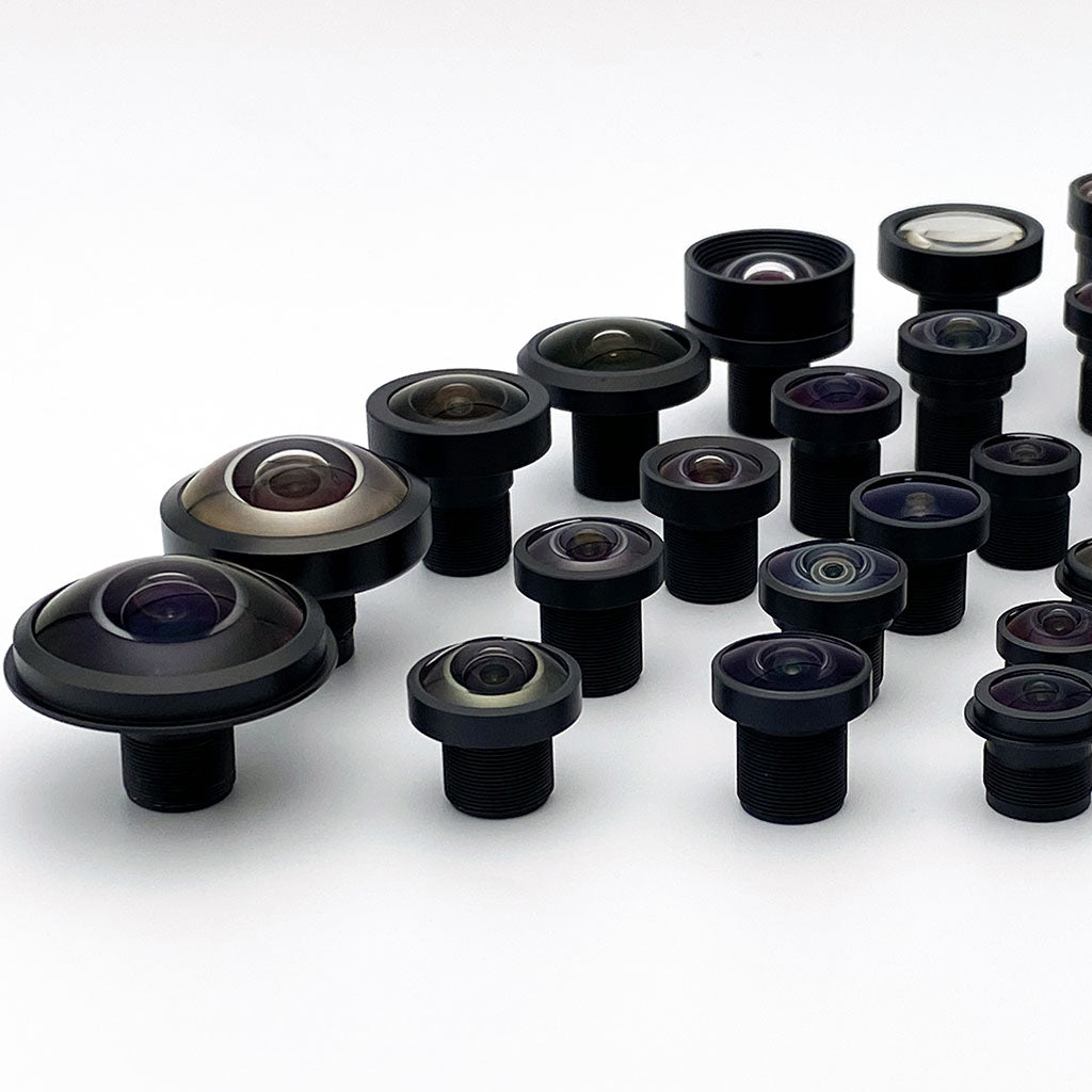
Focal length concentrates pixels on the feature; aperture decides where diffraction caps the system. These eight lenses cover both levers.

Lens picks by resolution requirement

Match a machine vision lens to the sensor's megapixel class and pixel pitch, not to a marketing label. The table pairs a verified Commonlands lens to each common resolution tier, from 1–2MP entry inspection through 8–12MP metrology, so the resolving-power and aperture picture stays honest against the Nyquist and diffraction tables above.

How we picked

Every rating below is taken from the lens datasheet and this article's own Nyquist and Airy-disk tables, not estimated. A lens rated for a higher megapixel class also satisfies a lower one, so the 8–12MP rows list the tightest pixel pitch each lens is published to support, while the entry tiers list the lowest-cost lens that covers the format. Where a pixel pitch is not published, the megapixel rating is given in the note instead.

Resolution tier Recommended lens Mount F# Smallest pixel pitch supported Note
1–2MP entry inspection CIL028 2.6mm M12 See product page Not the binding constraint at 1–2MP Rated 4K+, so resolving power is never the limit here. Pick the lowest-cost lens that covers your format.
5MP general purpose CIL059 6mm M12 F/1.7–F/5.6 See product page Rated 4–6MP wide open. Stopping to F/5.6 lifts the rating to 8–10MP as residual aberrations drop.
8–12MP embedded / automotive CIL368 7mm M12 F/1.8 2.0µm (IMX678) Fixed aperture. Covers 8MP automotive sensors to 1/1.7" with a 9.2mm image circle.
8–12MP inspection CIL160 16mm M12 F/1.9–F/5.6 See product page Fixed-aperture variants rated 12MP at F/2.8–F/4.0. The F/5.6 build drops to 8MP as diffraction grows.
8–12MP metrology CIL514 25mm C-mount F/2.8–F/16 3.45µm Adjustable iris. The Airy disk reaches two pixel pitches near F/5.6, the practical stop-down limit at 550nm.
8–12MP fine-pitch CIL535 35mm C-mount F/2.0–F/16 2.1µm Adjustable iris for 2.1–2.74µm pixels. Keep to F/4–F/5.6 to stay inside the pixel budget.

For sensors above 12MP on formats larger than about 1.1 inch, fixed-focal C-mount FA lenses from Kowa, Fujinon, and Moritex are the established choices. The Commonlands M12 and C-mount optics above target the 1/4" to 1.1" formats these tiers cover. Confirm any pick against the sensor's pixel pitch with the sensor size and lens compatibility guide and the working aperture with the f-number guide, then size the field of view in the FOV calculator.

Common mistakes when specifying resolution

A few specification errors show up again and again. Each traces back to treating one layer of the resolution chain as the whole answer.

  • Specifying megapixels without a field of view. Megapixels are a pixel budget, not a distribution. A 20MP camera behind a wide lens can deliver coarser mm per pixel at the part than a 5MP camera behind a telephoto. State pixel count and FOV together.
  • Treating 2 pixels as a detection threshold. Two pixels is the Nyquist floor, reachable only with near-perfect contrast and grid alignment. Design for 3 to 5 pixels minimum, and more for low-contrast defects.
  • Matching lens to sensor by megapixel label instead of pixel pitch and image circle. The label bundles two independent properties. Verify lp/mm against the Nyquist requirement and image circle against the sensor diagonal.
  • Stopping down for depth of field without checking the Airy disk. Past roughly two pixel pitches of diffraction blur, each additional stop trades away fine-detail contrast the algorithm needs. Compute d = 2.44 × λ × F/# before committing to F/11 or F/16.
  • Assuming uniform resolution across the frame. Corner MTF is lower than center MTF on many lenses, and distortion shifts local magnification. Verify performance at the image positions where defects actually appear.
  • Ignoring motion blur in the exposure budget. A system sized for a stationary target loses its margin when line-speed smear exceeds half a pixel. Check exposure time against velocity before finalizing the illumination spec.
  • Solving for detection when the task is measurement. Detection succeeds at 3 to 5 pixels; dimensional measurement typically needs 10 or more plus sub-pixel processing. Confirm which deliverable the downstream process expects.
Looking into a C-mount lens iris stopped down to a small polygonal aperture
A very small aperture sets the diffraction limit on resolution.

Frequently asked questions

What is spatial resolution in machine vision?

Spatial resolution is the real-world size represented by one pixel at the working distance, expressed in mm per pixel. Divide the field of view by the pixel count across it: a 100mm FOV on 2592 horizontal pixels gives 0.039mm per pixel. It sets the theoretical floor for the smallest detectable feature.

What is the minimum detectable size in machine vision?

Minimum detectable size is the smallest feature a vision system reliably identifies. Multiply spatial resolution by the pixels required across the feature: (FOV ÷ pixel count) × required pixels. A 100mm FOV on 2048 pixels gives 0.049mm per pixel, so a 5-pixel detection target means features of 0.24mm or larger.

What is IFOV in a camera?

IFOV (instantaneous field of view) is the angle subtended by one pixel: IFOV = FOV ÷ pixel count. A camera with an 80° horizontal FOV and 3840 pixels has an IFOV of about 0.021° per pixel, or 48 pixels per degree. Multiply IFOV in radians by working distance to get the pixel footprint on the object.

What does megapixel mean for a machine vision lens?

A megapixel rating describes the sensor class a lens is designed to cover, a combination of pixel pitch and format, not its optical resolving power. Resolving power is measured in lp/mm. Two lenses with different megapixel labels can resolve identically in lp/mm; the higher label often just reflects a larger image circle for a bigger sensor at the same pixel pitch.

What is the diffraction limit in machine vision?

The diffraction limit is the minimum blur spot a lens can produce at a given aperture, set by the wave nature of light. A diffraction-limited lens at F/8 and 550nm cannot resolve beyond roughly 227 lp/mm, and its Airy disk spans 10.7µm, more than three pixels on a 3.45µm sensor.

What is an Airy disk in optics?

The Airy disk is the bright central spot of the diffraction pattern formed when light passes through a circular aperture. Its diameter is d = 2.44 × wavelength × F-number, and it contains about 84% of the pattern's energy. It is the smallest blur spot any lens can produce at that aperture and wavelength.

How do I calculate mm per pixel?

Divide the field of view by the number of pixels across that dimension: mm per pixel = FOV (mm) ÷ pixel count. A 150mm FOV on 3840 horizontal pixels gives 0.039mm per pixel. The Commonlands field of view calculator outputs mm per pixel directly for any lens and sensor pair.

How many pixels do I need across a defect?

Two pixels is the Nyquist sampling floor, not a practical threshold. Use 3 to 5 pixels for high-contrast presence checks, 5 to 10 for shape classification, 8 to 15 for low-contrast defects, and 10 or more for dimensional measurement. Low contrast, noise, and motion blur push the requirement upward.

When does stopping down start hurting resolution?

Stopping down improves sharpness until residual aberrations fall below the Airy disk size, often between F/4 and F/8 on machine vision lenses. Past that point diffraction dominates: the Airy disk reaches two pixel pitches near F/5.6 on a 3.45µm sensor and near F/4 on a 2.74µm sensor.

Do I need a 12MP lens for a 12MP camera?

Not necessarily. Match pixel pitch and image circle, not labels. If a 5MP-rated lens resolves the lp/mm your pixel pitch demands and its image circle covers the sensor diagonal, it performs correctly on a 12MP camera. Check the sensor datasheet for pixel pitch first, then verify format coverage.

What is the Nyquist limit for machine vision lenses?

The Nyquist limit is the minimum resolving power a lens needs so the sensor sampling does not outrun the optics: lp/mm = 1 ÷ (2 × pixel pitch in mm). A 3.45µm pixel needs 145 lp/mm; a 2.74µm pixel needs 182 lp/mm. Below this, the lens blurs detail the sensor could capture.

How do blur and shutter speed affect defect detection?

Motion blur equals part velocity × exposure time. Keep it below half a pixel at your spatial resolution: maximum exposure = (0.5 × mm per pixel) ÷ velocity. At 200mm/s and 0.049mm per pixel, that is about 120µs. Longer exposures smear small defects across pixels and defeat the resolution budget.

What is the difference between spatial resolution and angular resolution?

Spatial resolution is physical size per pixel (mm per pixel) at a specific working distance. Angular resolution (IFOV) is angle per pixel, independent of distance. They are related by spatial resolution = working distance × IFOV in radians. Use angular resolution when working distance varies, spatial resolution for fixed inspection stations.

Match a lens to your resolution requirement

Send us the defect size, working distance, and sensor, and the Commonlands engineering team will work through the FOV, pixel coverage, lp/mm, and aperture numbers with you, or run the math yourself first.