
Depth of Field in Machine Vision: Aperture, Working Distance, and the Circle of Confusion
Aperture, focal length, working distance, and the circle of confusion decide how much of the scene stays sharp. This guide works through each one, shows where stopping down stops helping, and explains how depth of focus differs from depth of field.

Depth of field (DOF) in machine vision is the range of object distances that produce acceptably sharp images on the sensor. Four variables control it: f-number, focal length, working distance, and the permissible circle of confusion, which machine vision sets from pixel pitch rather than photographic convention. A larger working-distance-to-focal-length ratio extends DOF the most. Stopping down widens it further, until diffraction cancels the gain. Run your own numbers in the Commonlands camera depth of field calculator.
What is depth of field in machine vision?
Depth of field is the range of object distances over which a lens holds blur below the permissible circle of confusion on the sensor. In machine vision the blur limit comes from pixel pitch, not print sharpness, so practical DOF is far shallower than photography rules of thumb suggest. A published DOF figure needs a stated sharpness criterion and test conditions. That criterion can be a circle of confusion, measured MTF at a specified spatial frequency, or an application-resolution threshold.
An allowable circle of confusion defines geometric depth of field. It does not include diffraction or aberrations, so it cannot establish the full system's usable range. Check MTF through focus at the spatial frequencies needed for your task, especially when the in-focus diffraction blur is already close to the selected blur limit.
Geometry dominates: at low magnification DOF scales with the square of the working-distance-to-focal-length ratio, and F# and the CoC scale it linearly once the geometry is fixed. That is why a smaller pixel pitch, which tightens the CoC, shrinks the working DOF even though nothing about the lens changed. The working distance guide covers how WD fits the rest of the optical stack.

What determines depth of field in a machine vision system?
Four variables set depth of field: F#, focal length, working distance, and the permissible circle of confusion. To a low-magnification approximation, DOF grows with F# and CoC, and with the square of the working-distance-to-focal-length ratio. The exact near and far limits are nonlinear, and finite conjugates add pupil magnification through the working f-number.
Aperture (f-number)
Stopping down reduces the entrance pupil diameter, cutting off the marginal rays of the imaging cone. A defocused point then casts a smaller geometric blur spot, so a higher F# widens the sharp zone. At a fixed focal length, working distance, and blur budget, the widening is proportional to the working F#, and each stop halves the light.
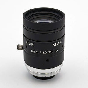
Many M12 lenses run at a fixed F#, so aperture is set at selection. An adjustable-iris C-mount lens such as the Commonlands CIL544 tunes it at the bench. See the f-number guide.
Focal length
At low magnification, well below hyperfocal focus, geometric DOF approximately scales with the inverse square of focal length at a fixed object distance and f-number: a 6mm lens holds roughly 7 times more DOF than a 16mm lens, since (16/6)² ≈ 7.1. The 6mm lens sees a wider field, though: moving the camera closer to match the 16mm framing restores approximately the same magnification and removes most of that DOF advantage.
If the feature size needs the longer lens, the extra DOF must come from aperture or working distance. See the focal length selection guide.
Working distance
DOF scales with the square of working distance, so moving the camera from 300mm to 600mm at constant focal length and aperture roughly quadruples it. Restoring the field of view needs a longer focal length, which cancels most of the gain at low magnification, so model the two together. Early on the camera can move, so a DOF problem is cheap to fix. Once the mechanics are committed, the remaining levers are optical.
Permissible blur (circle of confusion)
Relaxing the CoC raises the calculated DOF without changing the physical blur. Only the label of what counts as acceptable moves. The right CoC is the largest blur the algorithm still tolerates at full reliability. The section below gives per-task starting values.
Published DOF figures rarely state their CoC assumption. When comparing lenses, request the assumed CoC or recompute DOF from F#, focal length, and your own pixel-pitch CoC so the comparison is like for like.
Does stopping down the aperture increase depth of field?
Stopping down increases depth of field, and at a fixed focal length, working distance, and blur budget the geometric gain is proportional to the working F#. It costs light, and eventually the growing diffraction blur outweighs the added depth. On 1.5-2µm pixels, the Airy disk spans two pixel pitches by F/2.2-F/3 at 550nm, a gradual slide, not a fixed threshold.
Light loss
Each full stop halves the light, so going from F/2.8 to F/11, four stops, drops it to a sixteenth. Strobe power must rise or the exposure must lengthen, risking motion blur, and eventually the illumination system hits its power limit. Illumination is programmable, so the cost is often payable, but budget it.
Diffraction
Light passing through a small aperture spreads by diffraction, so the point image on the sensor becomes an Airy disk whose diameter grows with F#:
On 1.85µm pixels, an F/8 Airy disk at 550nm spans nearly 6 pixels, a blur floor under the entire image, so closing the iris past this point erases the resolution the extra DOF was meant to protect. The two-pitch marker falls near F/5.1 on 3.45µm pixels and near F/2.2 on 1.5µm pixels at the same wavelength.
It is a flag, not a limit: diffraction rises gradually across the band in use, so set the stop from system MTF or measured task performance, not spot diameter. The diffraction limit guide covers the resolution side.
Machine vision systems commonly operate in F/2.8-F/8. Commonlands can supply a measured through-focus MTF curve for a candidate lens, so the tradeoff is not left to the geometric estimate.
What circle of confusion should I use in machine vision?
Use a circle of confusion derived from pixel pitch, commonly 1-2 pixel pitches depending on the task. Pixel pitch comes from the sensor datasheet, not the format name. See the sensor size guide.
The machine vision criterion is CoC = k × pixel pitch, where k is the number of pixels of blur the task tolerates. The k values below are starting heuristics, not measured limits.
Sensor type shifts k as well. Monochrome sensors resolve at full pixel pitch, so k near 1 is a common measurement starting point. Bayer sensors are often given k near 2 because color interpolation already softens fine detail, but that is a convention, not a law: CFA, ISP, task, and system MTF set the real tolerance.
| Task | Starting CoC (pixels) | Rationale |
|---|---|---|
| Metrology, dimensional measurement | 1 | Use as an initial blur allowance, then measure edge-location error with the actual optics and algorithm |
| Fine surface inspection | 1 | Defects may span only 1-2 pixels. Blur masks them |
| Barcode, 2D code, OCR | 1-2 | Narrowest bar, cell edge, or stroke must stay resolved |
| Pick-and-place localization | 1-3 | Placement accuracy sets the tolerance |
| Presence detection, robot navigation | 2-4 | Features are large relative to pixel scale |
The definitive test is empirical: expose the real algorithm to controlled defocus at the working aperture and find where output error crosses the acceptance threshold. Enter that value, not a photography default, into the Commonlands depth of field calculator.
What is hyperfocal distance in machine vision?
Hyperfocal distance is the closest focus distance at which the far depth-of-field limit reaches infinity. For a thin lens H = f² / (N × c) + f, and the +f term is negligible at the distances below. Focused at H, everything from H/2 to infinity stays within the circle-of-confusion budget. It suits navigation and monitoring cameras with variable object distances, not fixed-distance inspection.
Because H scales with f², focal length dominates. With c = 3.7µm, two pixel pitches on a 1.85µm sensor, the Commonlands CIL821 2.1mm M12 lens at F/2.4 gives H = 2.1² / (2.4 × 0.0037) ≈ 0.50m. Everything from about 0.25m to infinity then holds within budget, a workable fixed-focus navigation camera. The CIL160 16mm at F/1.9 gives H ≈ 36m, near limit around 18m. Focus it at the working plane instead.
Hyperfocal focus fits AMR and drone navigation, wide-area monitoring, and factory-set fixed-focus modules, where object distances vary and no plane deserves peak sharpness. It is the wrong strategy for inspection, metrology, and barcode reading: at H/2 blur equals the full CoC, a liability when the target sits at one controlled distance. See the focusing guide for setting focus at either target.
The calculation is only as good as its CoC: tightening c from 6µm to 3µm doubles H and can push the near limit beyond the closest object the camera must see. Before committing a factory focus setting, verify the detection rate on images captured at H/2.
What is the difference between depth of focus and depth of field?
Depth of field is the object-side tolerance: how far the scene can move while lens and sensor stay fixed. Depth of focus is the image-side tolerance: how far the sensor can shift along the optical axis before blur exceeds the permissible circle of confusion, about 2 × the working F# × CoC in total. They are conjugates, not synonyms.
| Parameter | Depth of field | Depth of focus |
|---|---|---|
| Side of the system | Object side | Image side (sensor plane) |
| What moves | Object distance | Sensor position |
| Typical range | Millimeters to meters | Tens of micrometers |
| Failure signature | Parts at the wrong distance are blurry, others sharp | Entire image uniformly soft after assembly |
The image-side window totals about 2 × N_w × c, where the working f-number N_w = N × (1 + |m| / p) and p is the pupil magnification: roughly 40µm at F/4 with c = 5µm at low magnification, doubling at 1:1 when p = 1. Object-side depth of field grows as magnification falls, so a low-magnification system with generous depth of field still carries a tens-of-micrometers sensor-placement budget.
That window must absorb every sensor-position error in the build: PCB thickness variation, package height, flange tolerance, shims, and thermal drift, which can reach tens of micrometers in compact assemblies. A lens that passes bench testing can still image softly after integration, so validate focus in the assembled camera at the working aperture.
Which lenses fit depth-of-field-critical applications?
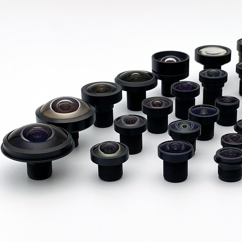
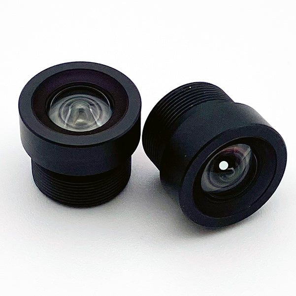
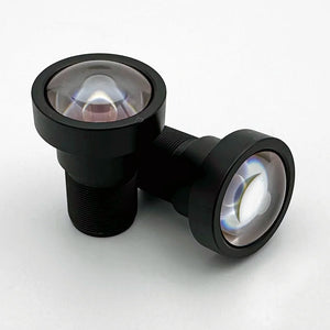
Short focal lengths give forgiving depth of field even at a fixed aperture. Longer focal lengths trade that margin for magnification, where a finite conjugate design holds sharpness at close working distances. The four M12 lenses below cover that range. Check the machine vision lens collection for current options. Commonlands ships in-stock lenses same day on orders placed before 12 PM PT.
All four are fixed-aperture designs, so the DOF decision is made when you pick the variant. Ordered by focal length.
| Rank | Lens | Mount | EFL | Aperture | When to choose it | Product |
|---|---|---|---|---|---|---|
| 1 | CIL059 | M12 | 5.9mm | F/1.7, F/2.8, F/4.0, F/5.6 fixed variants | Short-EFL layouts that need the widest DOF margin. The four fixed-aperture variants let the blur budget pick the F#. | Low distortion 6mm M12 lens |
| 2 | CIL064 | M12 | 6.0mm | F/2.9 fixed | Short-EFL DOF behavior on larger 1/1.6" to 2/3" sensors, covered by its 11.0mm image circle. | Two thirds inch 6mm M12 lens |
| 3 | CIL142 | M12 | 14.4mm (sold as 14.2mm) | F/2.6, F/4.1, F/5.2 fixed variants | Mid-telephoto framing where DOF tightens. The F/5.2 variant buys margin back when the light budget allows. | Telephoto 14.2mm M12 Lens |
| 4 | CIL121 | M12 | 21.8mm | F/2.8, F/5.9, F/8.0 fixed variants | Close-range telephoto work. Finite conjugate correction centered at 500mm holds sharpness where telephoto DOF is thinnest, and the F/8.0 variant maximizes it. | Telephoto 21.8mm M12 lens |

Technical references
Frequently asked questions
What is the circle of confusion in machine vision?
The circle of confusion is the maximum blur-spot diameter on the sensor that an application still treats as in focus. In machine vision it is an engineering tolerance set from pixel pitch and algorithm tolerance, commonly 1-2 pixel pitches, far tighter than photographic conventions for print viewing. Monochrome sensors often sit near 1 pixel pitch. Bayer RGB sensors are frequently allowed closer to 2, a demosaicing rule of thumb, not a law.
What is hyperfocal distance in machine vision?
Hyperfocal distance is the closest focus distance at which the far depth-of-field limit extends to infinity for a given lens, aperture, and circle of confusion. Focused at the hyperfocal distance H ≈ f² / (N × c), everything from H/2 to infinity stays within the blur budget. It suits navigation and monitoring cameras, not fixed-distance inspection.
What is depth of focus in machine vision?
Depth of focus is the allowed displacement of the image sensor along the optical axis before blur exceeds the permissible circle of confusion. It is an image-side tolerance, approximately 2 × the working F# × CoC in total, typically tens of micrometers. Depth of field is the corresponding object-side tolerance. The two are not interchangeable.
How do I increase depth of field in machine vision?
Raise the working-distance-to-focal-length ratio first, then stop down. Those two levers are coupled: shortening the focal length or backing the camera off only helps if you let the field of view widen, because restoring the original framing puts the ratio back. Stopping down costs light and adds diffraction blur. Model the options in the Commonlands depth of field calculator before changing hardware.
When does diffraction cancel the benefit of a smaller aperture?
Gradually, as the Airy disk grows past the sensor pixel pitch, with no single crossover point. The Airy disk diameter is approximately 2.44 × wavelength × F#: about 10.7µm at F/8 in 550nm light, which spans nearly 6 pixels on a 1.85µm sensor. Larger pixels, such as 3.45µm, tolerate a higher F# before diffraction dominates.
Should I focus at the working plane or hyperfocal distance?
Focus at the working plane when the target sits at a defined, repeatable distance, which covers most inspection systems. Focus at the hyperfocal distance when object distances vary continuously and no single plane dominates, as in robot navigation, wide-area monitoring, and fixed-focus embedded cameras.
Need a DOF budget reviewed?
Commonlands manufactures M12 and C-mount lenses for machine vision, with MTF testing as part of production quality control. Send the San Diego engineering team your working distance, part-height variation, and sensor, and we will recommend a lens and operating aperture. In-stock samples ship same day on orders placed before 12 PM PT.